
Kinship identification based on rare severe variants from trio whole exome sequencing
Introduction
Whole exome sequencing (WES) is the sequencing of all exons in genomic DNA. With the successful application of WES in scientific research and clinical practice, WES has been widely recognized to identify pathogenic variations in patients with genetic disorders, which could facilitate the diagnosis and clinical decision-making processes (1,2). WES would identify hundreds of thousands of variants in one sample (3,4). Generally, the pathogenic mutations could not be effectively identified by WES data from the proband alone (5-7). In contrast, WES data from other family members (i.e., family WES) can help to effectively identify the pathogenic mutations by familial co-segregation analysis (7,8). For example, WES data of a proband and his parents (first-degree relatives) can trace the origin of the proband’s variant (de novo, from father, from mother) to assess its pathogenicity based on the gene’s inheritance model (8). For some cases, WES data of a proband’s second-degree relatives are needed. For example, Prader-Willi syndrome and Angelman syndrome are caused by variants on imprinted genes expressed in either paternal or maternal alleles, including large-sized SV (9) and small Indels (10). Pathogenicity of a mutation on an imprinted gene needs to be evaluated by variant data from a pedigree including the proband, his parents and his grandparents (second-degree relatives) (11,12). In other cases where there are multiple patients exist in a large pedigree, WES data of affected relatives (may be three-degree relatives) are also important to assess the potential pathogenicity of the proband’s variants (8,13). Analysis of these pedigree-based WES data relies on correct kinships record among the sequenced samples (7,14). However, kinships labeling mistakes could not be completely avoided, especially for pedigrees from the same sequencing batch. For example, an average of 120 pedigree data will be sent to the Molecular Medical Center of Children’s Hospital of Fudan University for WES every week. Sample swap events may occur among different families or within the same family during processes of sample collection, labeling or delivery. Error kinships caused by sample swaps may delay diagnosis or clinical decision. Therefore, it is an important quality-control step in clinical molecular diagnosis to accurately identify kinships of members from large-scale WES samples.
Previously, the Molecular Diagnosis Center of the Children’s Hospital of Fudan University has developed a WES data analysis and clinical diagnosis pipeline (Fudan Pipeline 2.0) (15). This protocol automatically annotates and filters the variation data obtained from WES and finally obtains a list of candidate pathogenic variants for manual interpretation by genetic analysts. When applied in trio WES, the Fudan Pipeline would use the pedigree information to evaluate the pathogenicity. Thus, a quality control module to identify and double check kinship is essential for the pipeline.
On the basis of Fudan Pipeline 2.0, we automatically identified the kinships among samples by evaluating the similarity of variant data obtained from WES. In this study, the similarity among samples was assessed and compared two methods: using the total variants data of WES and by rare, severe variation data (abbreviated as feature variants) selected by Fudan Pipeline 2.0 (technically, with capture region selection, population frequency filtration and variant damage prediction). Results show that similarity scores based on total variant could not accurately identify the kinship among samples. In contrast, similarity scores based on feature variants could not only identify the kinship between two samples accurately but also identify the kinship levels (first-, second-, and third-degree) among samples.
Methods
Sources of family samples
By now, these have been a total of 2,870 families performed WES (Captured Kit: Agilent Sureselect All Exons Human V5, Sequencing Platform: Illumina Hiseq 2000). Among 2,870 families, 2,735 are core families (including three members: the proband and the parents), 130 are composed of proband, parents, and siblings, 4 are composed of proband, parents and other family members up to second-degree relatives, and 1 includes third-degree relatives as the farthest relatives. In this study, 100 random core families and all 5 families with second- or third-degree relatives were selected with informed consent. The random selection procedure was performed as following: first, all core families were numbered from 1 to 2,735; second, 100 integers were extracted from 1 to 2,735 by a random seed generator in R program, and families whose numbers correspond to these 100 integers were the enrolled families.
Sources of total variants
After removed of adapters and low-quality reads, WES reads were mapped to human reference genome (hg19). After local re-alignment and base recalibration by GATK software (16,17), Picard (http://picard.sourceforge.net/index.shtml) was used to remove the redundant sequences generated by PCR amplification during library construction. Finally, GATK software was used for variant calling after removing redundant reads, producing variant call format (VCF) files. Sequencing and variant calling procedures were performed by a CLIA-certified laboratory (CLIA license: 99D2064856) of WuXi NextCODE Genomics (Shanghai) Co., Ltd.
Variant screening
In this study, feature variants were defined as variants obtained after following filtrations in Fudan Pipeline 2.0: capture region, population allele frequency, and the predicted influence on proteins. In details, the capture region filtration would filter out all variations 15 bp or more away from the splicing junctions except for pathogenic variants reported in HGMD or ClinVar. The population allele frequency filtration would exclude variants reported as homozygous or with high allele frequency in public or local databases. The public databases include the 1,000 Genomes Project (http://www.1000genomes.org), the ExAC (http://exac.broadinstitute.org) and the gnomAD (http://gnomad.broadinstitute.org). Variants with more than 5 homozygous records or AF higher than 5% would be excluded. Local population database was built based on all 2870 WES trios in this center. Variants with local frequency greater than 2% would be further excluded. Protein-damaging of variants were annotated by ANNOVAR (18) and VEP (19), including damage prediction for missense mutations and annotation of frameshift mutation, splice site mutation and nonsense mutation.
Calculation of sample similarity
The sample similarity was measured based on variant overlapping between samples. Let S1 and S2 be the set of variants in sample 1 and sample 2, respectively. Then their similarity was defined as:
For feature variants,
For total variants, we used RTG Tools (Version 3.9) (20) for the calculation. The sensitivity value and precision value from the output file of RTG Tools equal to Sim(S1→S2) and Sim(S2→S1), respectively. Variants on autosomes and sex chromosomes were both included.
Kinship identification based on feature variants during WES
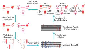
After performing WES, total variants were identified with standard variant calling process [BWA (21) and GATK golden practice (16,17)], and the feature variants were selected with Fudan Pipeline 2.0 (15). Sample similarity was calculated based on the feature variants, and then the kinships among the samples were deduced in a single-blinded manner (the person performing the analysis has no prior knowledge of the relationship between the assessed pairs). If the kinships did not match the laboratory records, the real kinship would be double confirmed with sample identification and follow-confirmation (Figure 1).
Ethics approval
The genetic testing was approved by the ethics committees of Children’s Hospital, Fudan University (2014-107 and 2015-130). Informed consents were obtained from patients’ parents prior to the start of the study.
Results
General data of the included family samples
A total of 105 families were included, among which 100 families were core families, 4 families were composed of second-degree relatives as farthest relatives, and 1 family was composed of the third-degree relatives as the farthest relatives. In total there were 323 samples from 51 sequencing batches. Among the 105 probands, 66 were males and 39 were females. The first-degree kinships were defined as relationships between children and parents or relationships among children. The second-degree kinships included: proband/sibling and aunt/uncle, proband/sibling and grandparents. The third-degree kinships included: proband/sibling and cousin. Other kinships were treated as unrelated. The numbers of sample pairs corresponding to the first-, second-, and third-degree kinships were 223, 9, and 2 respectively, and the numbers of unrelated sample pairs were 51,769.
Numbers of total variants and feature variants
Among the 323 samples, the average number of total variants was 111,900 (range: 99,820–120,600). With Fudan Pipeline, 60,890–81,840 variants were filtered out during capture region filtration in Fudan Pipeline, 36,200–38,580 variants were filtered out by population frequency filtration, and 510–922 variants were filtered out after variation damage annotation. Finally, the average number of feature variants per sample was 688 (range: 594–778).
Distribution of sample similarity
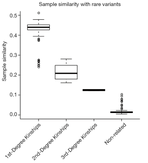
The distribution of sample similarity calculated with total variants is shown in Figure 2A. The sample similarities ranges for the first-, second-, and third-degree kinships were 0.319–0.784, 0.290–0.700, and 0.664–0.670 (only two values), respectively. Due to the overlap of sample similarities based on total variants, 17.5% of the first-degree kinships could not be distinguished from the second-degree, and all the third-degree kinships could not be distinguished from the second-degree. In addition, the similarity between unrelated samples ranged from 0.273 to 0.654, which were overlapped with the first-degree and second-degree kinships. Therefore, the sample similarity based on total variant calculation could not accurately identify whether two samples were related. In contrast, the sample similarity based on feature variants among first-degree kinships ranged from 0.254 to 0.449, the second- and third-degree kinships were 0.129–0.217 and 0.097–0.098 (only two values), respectively. Moreover, the similarity between unrelated samples was 0–0.045 (Figure 2B), which makes 0.05 a powerful threshold to distinguish related and unrelated samples. For related sample pairs, 0.25 could be used as threshold values to distinguish between the first- and the second-degree kinships; 0.1 could be used as threshold values to distinguish between the second- and the third-degree kinships (Figure 2B). Three thresholds used to distinguish kinships were marked on Figure 2B.
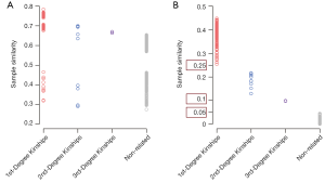
We also investigated the distribution of sample similarity with rare variant, which including the rare synonymous SNVs. As shown in Figure S1, the first-degree kinships could not be clearly separated with secondary kinships. The result indicated that both allele frequency and severity were important for feature variants selection.
Identification of kinship based on sample similarity
Cluster analysis of samples was performed based on the sample similarity to test whether the whole pedigree tree could be reconstructed. Based on total variants, members in 21 families (20%) would be reconstructed incorrectly (Figure 3A, marked in red). The incorrect cases included clustering multiple core families into a large group (hereafter referred to as large families) or splitting the same family into multiple families or single individual. Among them, 15 core families were clustered into three large families (Figure 3A, Large Family No 1, No 2 and No 3, marked in red), and 21 individuals coming from 6 families were wrongly split into 18 clusters. In contrast, sample similarity based on feature variants could accurately cluster family members and distinguish different families (Figure 3B). In addition, sample similarity based on feature variants could identify correct kinships for complex families. As shown in Tables 1 and 2, the kinship of a 6-member family (family code: 101) and a 5-member family (family code: 102) could be correctly predicted by the sample similarity based on feature variants, providing results which was identical with laboratory sample records.
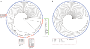
Table 1
| Relation with the proband | Relation with the proband | Sample similarity | Kinship suggested by similarity |
|---|---|---|---|
| Proband himself/herself | Sister | 0.448 | First-degree |
| Proband himself/herself | Father | 0.397 | First-degree |
| Proband himself/herself | Mother | 0.367 | First-degree |
| Proband himself/herself | Aunt | 0.171 | Second-degree |
| Proband himself/herself | Cousin | 0.097 | Third-degree |
| Sister | Father | 0.396 | First-degree |
| Sister | Mother | 0.368 | First-degree |
| Sister | Aunt | 0.183 | Second-degree |
| Sister | Cousin | 0.098 | Third-degree |
| Father | Mother | 0.013 | None |
| Father | Aunt | 0.014 | None |
| Father | Cousin | 0.015 | None |
| Mother | Aunt | 0.364 | First-degree |
| Mother | Cousin | 0.200 | Second-degree |
| Aunt | Cousin | 0.359 | First-degree |
Table 2
| Relation with the proband | Relation with the proband | Sample similarity | Kinship suggested by similarity |
|---|---|---|---|
| Proband himself/herself | Mother | 0.406 | First-degree |
| Proband himself/herself | Father | 0.410 | First-degree |
| Proband himself/herself | Aunt | 0.217 | Second-degree |
| Proband himself/herself | Grandmother | 0.213 | Second-degree |
| Mother | Father | 0.009 | None |
| Mother | Aunt | 0.439 | First-degree |
| Mother | Grandmother | 0.336 | First-degree |
| Father | Aunt | 0.020 | None |
| Father | Grandmother | 0.005 | None |
| Aunt | Grandmother | 0.344 | First-degree |
An example of applications
By using the data of two families simulated with sample swaps, we described the application of the feature variant-based similarity calculation method, which not only can distinguish sample swap between families but can also identify sample swap within a family. Sample swap event was simulated between a 6-person family (family code: 101) and a 5-person family (family code: 102) included in this study. The simulations included: (I) an interchange of the fathers of two families presenting inter-family swap; and (II) an interchange of mother and aunt in Family 101 presenting intra-family swap.
Based on sample similarity calculated by feature variants, 101F (father of Family 102 but labeled as father of Family 101) was clustered with the members of Family 102, whereas 102F (the father of Family 101 but labeled as father of Family 102) was clustered with the members of Family 101 (Figure 4). Sample similarities suggested that there was a sample swap between 101F and 102F (Figure 4), and helped to correctly reconstruct the original kinships. In addition, the kinships suggested by sample similarity showed first-degree kinships between Mother and Cousin (101M and 101CS) as well as between Proband/Sister and Aunt (101P/101S and 101A). On the other hand, second-degree kinships were identified between Proband/Sister and Mother (101P/101S and 101M) as well as Cousin and Aunt (101CS and 101A) (Tables 3,4). Therefore, a swap between mother and aunt was identified. The above results suggested that the feature variant-based calculation of sample similarity can accurately identify swapped samples from both inter-family and intra-family.
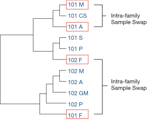
Table 3
| Relation with the proband | Relation with the proband | Sample similarity | Kinship suggested by similarity |
|---|---|---|---|
| Proband himself/herself | Sister | 0.448 | First-degree |
| Proband himself/herself* | Father | 0.007 | None |
| Proband himself/herself* | Mother | 0.171 | Second-degree |
| Proband himself/herself* | Aunt | 0.367 | First-degree |
| Proband himself/herself | Cousin | 0.097 | Third-degree |
| Sister* | Father | 0.001 | None |
| Sister* | Mother | 0.183 | Second-degree |
| Sister* | Aunt | 0.368 | First-degree |
| Sister | Cousin | 0.098 | Third-degree |
| Father | Mother | 0.007 | None |
| Father | Aunt | 0.005 | None |
| Father | Cousin | 0.004 | None |
| Mother | Aunt | 0.364 | First-degree |
| Mother* | Cousin | 0.359 | First-degree |
| Aunt* | Cousin | 0.200 | Second-degree |
The row labelled with * indicates that the kinships suggested by sample similarity do not correspond to the kinships in the laboratory records.
Table 4
| Relation with the proband | Relation with the proband | Sample similarity | Kinship suggested by similarity |
|---|---|---|---|
| Proband himself/herself | Mother | 0.406 | First-degree |
| Proband himself/herself* | Father | 0.001 | None |
| Proband himself/herself | Aunt | 0.217 | Second-degree |
| Proband himself/herself | Grandmother | 0.213 | Second-degree |
| Mother | Father | 0.008 | None |
| Mother | Aunt | 0.440 | First-degree |
| Mother | Grandmother | 0.336 | First-degree |
| Father | Aunt | 0.009 | None |
| Father | Grandmother | 0.011 | None |
| Aunt | Grandmother | 0.344 | First-degree |
The row labelled with * indicates that the kinships suggested by sample similarity do not correspond to the kinships in the laboratory records.
Discussion
In our current study, analysis of WES data of 323 samples from 105 families in the sample bank of the Molecular Diagnosis Center of Children’s Hospital of Fudan University showed that the total variants by WES could not accurately identify the kinships among samples. In contrast, the feature variants filtered by capture region, population frequency and damage annotation could accurately reconstruct the kinships of 323 samples.
Compared with other researches, this study focuses on not the general kinship identification. Instead, the application is applied on a targeted question: how to efficiently identify kinship in NGS samples, provided with no further data and routinely increasing samples. Many methods prefer pre-designed SNP panel or well-constructed genotype data. In this study, we only use allele frequency and the potential protein-damaging evaluation of variants, which were part of data analysis process for genetic diagnosis. Thus, in practise, no further data preparing process was needed. We tested other methods, such as KING for kinship inference. The input file takes 40 minutes to prepare, and needs to be re-prepared if new sample is added in the cohort. For specified kinship identification requirement (that is, identification kinship from WES trio cohort), this study proposed a targeted solution that requires no further experiment or repeated data preparation.
The sample similarity calculated by WES feature variants has many practical values. First, the concept can be easily understood by genetic analysts. The similarity directly reflects the consistency of rare and potential protein-damaging variants between two samples. Second, because such similarity score can distinguish different kinships, it could be used as kinship quality control module to correct potential sample swap cases in time. For example, the threshold value 0.05 can be used to distinguish the presence or absence of kinship between samples. The similarity lower than 0.05 between samples in a family or higher than 0.05 between samples from two families indicates an inter-family sample swap to have occurred (as described in 2.5), which should be corrected before genetic analyze. Alternatively, the sample similarity could also identify biological parents, which helps the genetic analysts to decide how to perform the familial co-segregation analysis. Notably, more than 99% of the families performing WES in our center are core families composed of probands and parents, so the lakes of adequate samples of second- or third-degree kinship for the study. Although our current study indicated that 0.25 and 0.1 could also be used as similarity thresholds to distinguish first, second, and third-degree kinships, further tests were still needed in larger families.
For a targeted kinship identification method, here are some limitations. First, it works better with population-related allele frequency. Although public databases are providing population-specific allele frequency data, a local database to exclude population bias were always suggested. Second, it was designed for single data type. If samples were sequenced by different platform, the feature variants might be influenced by system bias. Third, this study was based on limited number of WES data, which need more replication studies for further application. Fourth, this study chose to filter variants with high allele-frequency and treat rare-variants equally. A further allele frequency-based weightage might help to improve the identification outcome.
In this study, the kinship identification process based on trio WES feature variants was used as the kinship quality control module in Fudan Pipeline (15). With this module, both time and cost could be saved for family data re-analysis caused by sample swap events.
Acknowledgments
Funding: This work was funded by Shanghai Sailing Program (16YF1401000, 18YF1402500), National Key Research and Development Program (2016YFC0905102, 2018YFC0116903), the Shanghai Hospital Development Center (SHDC 12017110), Science and Technology Commission of Shanghai Municipality (16ZR1446500), National Natural Science Fund of China (31701152, 31701138) and Research Projects of the Shanghai Municipal Health and Family Planning Committee (20174Y0026), Shanghai Key Laboratory of Birth Defects (13DZ2260600).
Footnote
Conflicts of Interest: All authors have completed the ICMJE uniform disclosure form (available at http://dx.doi.org/10.21037/pm.2019.05.03). WHZ serves as an unpaid executive editor-in-chief of Pediatric Medicine. The other authors have no conflicts of interest to declare.
Ethical Statement: The authors are accountable for all aspects of the work in ensuring that questions related to the accuracy or integrity of any part of the work are appropriately investigated and resolved. The study was conducted in accordance with the Declaration of Helsinki (as revised in 2013). The genetic testing was approved by the ethics committees of Children’s Hospital, Fudan University (2014-107 and 2015-130). Informed consents were obtained from patients’ parents prior to the start of the study.
Open Access Statement: This is an Open Access article distributed in accordance with the Creative Commons Attribution-NonCommercial-NoDerivs 4.0 International License (CC BY-NC-ND 4.0), which permits the non-commercial replication and distribution of the article with the strict proviso that no changes or edits are made and the original work is properly cited (including links to both the formal publication through the relevant DOI and the license). See: https://creativecommons.org/licenses/by-nc-nd/4.0/.
References
- Miller NA, Farrow EG, Gibson M, et al. A 26-hour system of highly sensitive whole genome sequencing for emergency management of genetic diseases. Genome Med 2015;7:100. [Crossref] [PubMed]
- Yang Y, Muzny DM, Reid JG, et al. Clinical whole-exome sequencing for the diagnosis of mendelian disorders. N Engl J Med 2013;369:1502-11. [Crossref] [PubMed]
- Pelak K, Shianna KV, Ge D, et al. The characterization of twenty sequenced human genomes. PLoS Genet 2010;6:e1001111. [Crossref] [PubMed]
- Li MX, Kwan JS, Bao SY, et al. Predicting mendelian disease-causing non-synonymous single nucleotide variants in exome sequencing studies. PLoS Genet 2013;9:e1003143. [Crossref] [PubMed]
- Smedley D, Jacobsen JO, Jager M, et al. Next-generation diagnostics and disease-gene discovery with the Exomiser. Nat Protoc 2015;10:2004-15. [Crossref] [PubMed]
- MacArthur DG, Balasubramanian S, Frankish A, et al. A systematic survey of loss-of-function variants in human protein-coding genes. Science 2012;335:823-8. [Crossref] [PubMed]
- Heinrich V, Kamphans T, Mundlos S, et al. A likelihood ratio-based method to predict exact pedigrees for complex families from next-generation sequencing data. Bioinformatics 2017;33:72-8. [Crossref] [PubMed]
- Bamshad MJ, Ng SB, Bigham AW, et al. Exome sequencing as a tool for Mendelian disease gene discovery. Nat Rev Genet 2011;12:745-55. [Crossref] [PubMed]
- Kim SJ, Miller JL, Kuipers PJ, et al. Unique and atypical deletions in Prader-Willi syndrome reveal distinct phenotypes. Eur J Hum Genet 2012;20:283-90. [Crossref] [PubMed]
- Runte M, Kroisel PM, Gillessen-Kaesbach G, et al. SNURF-SNRPN and UBE3A transcript levels in patients with Angelman syndrome. Hum Genet 2004;114:553-61. [Crossref] [PubMed]
- Ming JE, Blagowidow N, Knoll JH, et al. Submicroscopic deletion in cousins with Prader-Willi syndrome causes a grandmatrilineal inheritance pattern: effects of imprinting. Am J Med Genet 2000;92:19-24. [Crossref] [PubMed]
- Bürger J, Horn D, Tonnies H, et al. Familial interstitial 570 kbp deletion of the UBE3A gene region causing Angelman syndrome but not Prader-Willi syndrome. Am J Med Genet 2002;111:233-7. [Crossref] [PubMed]
- Wells QS, Becker JR, Su YR, et al. Whole exome sequencing identifies a causal RBM20 mutation in a large pedigree with familial dilated cardiomyopathy. Circ Cardiovasc Genet 2013;6:317-26. [Crossref] [PubMed]
- Riordan JR, Rommens JM, Kerem B, et al. Identification of the cystic fibrosis gene: cloning and characterization of complementary DNA. Science 1989;245:1066-73. [Crossref] [PubMed]
- Yang L, Dong XR, Peng XM, et al. Evaluation of turn around time and diagnostic accuracy of the next generation sequencing data analysis pipeline version 2 of Children's Hospital of Fudan University. Chin J Evid Based Pediatr 2018;13:118-23.
- McKenna A, Hanna M, Banks E, et al. The Genome Analysis Toolkit: a MapReduce framework for analyzing next-generation DNA sequencing data. Genome Res 2010;20:1297-303. [Crossref] [PubMed]
- Van der Auwera GA, Carneiro MO, Hartl C, et al. From FastQ data to high confidence variant calls: the Genome Analysis Toolkit best practices pipeline. Curr Protoc Bioinformatics 2013;43:11.10.1-33.
- Wang K, Li M, Hakonarson H. ANNOVAR: functional annotation of genetic variants from high-throughput sequencing data. Nucleic Acids Res 2010;38:e164. [Crossref] [PubMed]
- McLaren W, Pritchard B, Rios D, et al. Deriving the consequences of genomic variants with the Ensembl API and SNP Effect Predictor. Bioinformatics 2010;26:2069-70. [Crossref] [PubMed]
- Cleary JG, Braithwaite R, Gaastra K, et al. Comparing Variant Call Files for Performance Benchmarking of Next-Generation Sequencing Variant Calling Pipelines. Available online: https://www.biorxiv.org/content/biorxiv/early/2015/08/02/023754.full.pdf
- Li H, Durbin R. Fast and accurate short read alignment with Burrows-Wheeler transform. Bioinformatics 2009;25:1754-60. [Crossref] [PubMed]
Cite this article as: Qin Q, Li ZX, Wu BB, Wang HJ, Dong XR, Lu YL, Zhou WH. Kinship identification based on rare severe variants from trio whole exome sequencing. Pediatr Med 2019;2:19.

